Nord Stream Long Distance Gas Pipeline – Part 3
Application of Basic and AGA equations for estimating maximum gas flow in a long-distance pipeline
By:
Jay Rajani, Ph.D., Kindra Snow-McGregor, P.E., Mahmood Moshfeghian, Ph.D.
Introduction
Following on the previous two TOTMs [1, 2] on Nord Stream long distance pipeline for natural gas transmission from Russia to Europe, this TOTM discusses the application of various long distance gas transmission correlations/equations that are available to determine the maximum gas capacity of a long-distance pipeline. In addition, calculations can be done to estimate the line packed gas volume; demonstrating that a long-distance pipeline can be used as a gas storage facility as well.
Case Study Data
In the previous TOTMs, we discussed various parameters that are available in the public domain [3] and presented in Table 1. Nord Stream 1 has 2 parallel gas pipelines, each pipeline capable of transporting gas from Russia to Germany at a rate of 75.34 million Std m3/day (2660.6 MMSCFD)
Table 1. Pipeline Specifications in SI and FPS Units

As the composition of the gas transported in the NS1 pipelines has not published, it was assumed for this study that the Norwegian gas, shown in Table 2, that is transported to the European Continental Shelf would be a good representation of the gas in the NS1 pipeline.
Table 2. Composition of the feed gas

Based on the above data, the physical and flow properties values were calculated and presented in Tables 3 and 4 in SI and FPS units, respectively.
Table 3. Calculated results for gas at a rate of 75.34 million Std m3/day

Table 4. Calculated results for gas at a rate of 2660.6 MMSCFD

In this study, two standard equations derived from the basic gas flow equation reflecting the average (mean) conditions have been used to estimate the NS1 pipeline capacity. These relationships are the BASIC and AGA (American Gas Association) equations containing a friction factor “f”. These equations are [4]:

The AGA equation estimates the friction factor under two conditions, “partially turbulent” and “fully turbulent”. The “partially turbulent” correlation is the Colebrook-White equation for smooth pipe. The smooth pipe assumption is corrected using a drag factor, Ff, which accounts for several pipeline characteristics: pipe wall condition, welds, changes in the direction of gas flow, isolation valves, etc. In the “fully turbulent” region the friction factor is independent of Reynolds number and depends only on the dimensionless roughness of the pipe.
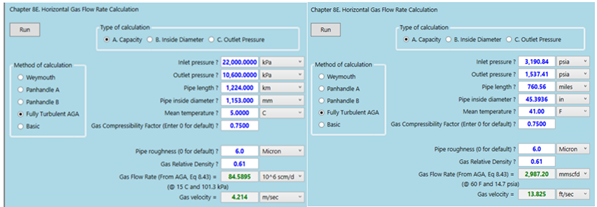
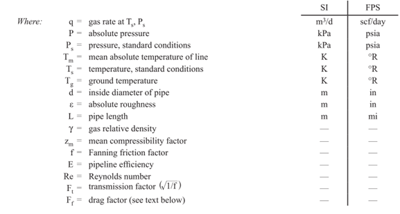
These equations are available in GCAP software [5] and the screenshot of GCAP results are presented in Figures A1 – A5 in Appendix A.
Table 5. Calculated results for gas at a rate of 75.34 million Std m3/day

Table 6. Calculated results for gas at a rate of 2660.6 MMSCFD

The BASIC equation estimated gas flow of 84.07 million Std m3 (2969 MMscfd) of gas assuming 100 % efficiency. The BASIC equation estimated gas flow of 75.63 million Std m3 (2671 MMscfd) assuming 90 % efficiency.
The AGA equation estimated a gas flow of 84.59 million Std m3 of gas (2987 MMscfd) assuming 100% efficiency.
The published capacity of NS1 pipeline is 75.34 million Std m3 of gas [3].
A design flow rate check was also initiated by using PROMAX [6] that uses the single-phase regimes and single-phase basic equation applying Colebrook friction factor. This methodology gave a flow rate of 83.1 million Std m3 of gas.
The differences between the estimated and actual are 0.4% for 90% Basic, 11.6% for 100% BASIC, 12.30% for AGA and 10.3% with PROMAX. Considering that the gas composition is not known for NS1, these differences are reasonable.
Pipe Wall Thickness
NS1 pipeline is varying in operating pressure, thus varying pipeline thickness. Using Barlow’s formula, a check on the wall thickness was made. Barlow’s formula relates the internal pressure that a given pipe can withstand as a function of its dimensions and strength of its material.
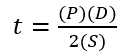
Where:
t = pipe wall thickness, mm (in)
P = 1.1 x design pressure, MPag (psig)
S = allowable stress, 483 MPag (70,000 psi) for grade x70 steel
D = outside diameter, mm (in)
In the Barlow’s formula, there is no provision of corrosion allowance. If we include this in the Barlow’s formula and take 3 mm as corrosion allowance (ca), then

Using Barlow’s equation, the pipeline wall thickness for different segments were calculated and presented in Table 7.
Table 7. Estimated pipeline wall thickness for different segments

Table 7 shows calculated pipeline wall thickness (t) with a corrosion allowance, ca. This information reveals a good agreement with the published data is reached using Barlow’s formula.
Line Packing
The NS1 gas pipeline can also be used to store gas when not used for gas transport. The methodology to determine how many standard cubic meters of gas can be held is given below.
Inventory (V) of gas pipeline can be calculated with:
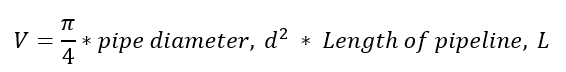
Taking the internal diameter of the pipeline as 1.153 m (3.78 ft) and pipeline length of 1 224 000 m (4 015 748 ft), the pipeline volume is 1 277 997 m3 (12 578 711 ft3).
Then using the real gas law:
PV = nZRT
or molar volume

Where P is the average pressure between inlet (22000 kPa or 3190 psia) and outlet (10600 kPa or 1537 psia) pressures amounting to 16300 kPa (23663 psia), T is the average temperature in the pipeline (5 ⁰C=41°F or 278 K=500.4 °R), Z is the average compressibility of 0.75 and R is the universal gas constant (8.314 kPa.m3/kmol. K or 10.732 psia.ft3/lbmol-°R).
n = 12 017 147 kmol (26 497 809)
Now 1 kmol = 23.64 Std m3 and 1 lbmol = 379.5 scf
Then the amount of standard cubic meters of gas that can be line-packed is 284.1 million Std m3 (10.6x10⁹ scf).
This is the amount of gas that can be stored in the pipeline when it is not operating in the transportation phase.
Concluding Remarks
The methodology used above demonstrates how standard long distance pipeline flow correlations/equations (BASIC and AGA equations) can be used in evaluating the design flow rates of an installed or of an operating pipeline. It was noted that the Basic equation with 90%-line efficiency matched the published design capacity very closely.
Pipe wall thickness calculation methodology using Barlow’s formula also shows good agreement with that of published data.
In addition, using the real gas law, it can be demonstrated that considerable amount of gas can be line-packed when the pipeline is in non-transportation mode.
To learn more about similar cases and how to minimize operational problems, we suggest attending our G4 (Gas Conditioning and Processing), P81 (CO2 Surface Facilities), and PF4 (Oil Production and Processing Facilities) courses.
References:
1. Moshfeghian, M., Rajani, J., and Snow-McGregor, K., “Transportation of Natural Gas in Dense Phase – Nord Stream”, PetroSkills TIP OF THE MONTH, April 2022.
2. Langer, J.F, Snow-McGregor, K, and Rajani, J., “Part 2: Nord Stream Pipelines – Multiple Parallel Paths to Succes or Failure?”, PetroSkills TIP OF THE MONTH, April 2022.
3. Beaubouef, B., “Nord stream completes the world’s longest subsea pipeline,” Offshore, P30, December 2011.
4. Campbell, J.M., “Gas Conditioning and Processing, Volume 1: The Fundamentals,” 9th Edition, 3rd Printing, Editors Hubbard, R., and Snow–McGregor, K., Campbell Petroleum Series, Norman, Oklahoma, PetroSkills 2018
5. GCAP 10.2.1, Gas Conditioning and Processing, PetroSkills/Campbell, Tulsa, Oklahoma, 2022.
Appendix A: GCAP Results
Figure A1. Calorimetric Values
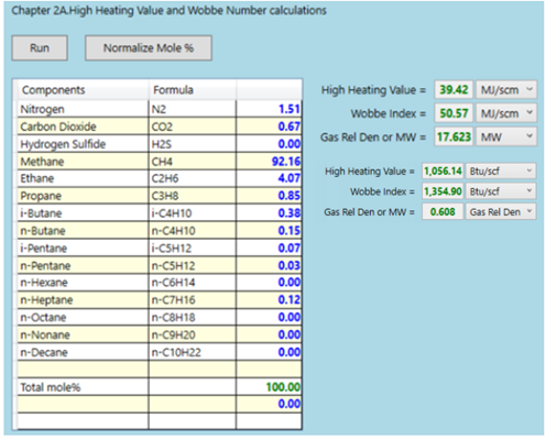
Figure A2. Average gas density by GCAP-Option 3C, SRK EOS

Figure A3. Estimated design pipeline capacity by basic Equation with 90 % efficiency

Figure A4. Estimated design pipeline capacity by basic Equation with 100 % efficiency

Figure A5. Estimated design pipeline capacity by AGA Equation