Overview of Gas – Lift; Part 2: Operational Fundamentals for the Performance of a Gas Lift Well, Related to Choke Flow, Single Phase Gas, and Multiphase Flowing Gradients.
By: Frank E. Ashford, Ph.D., PetroSkills Senior Advisor
Wes H. Wright, PetroSkills Senior Advisor
I) Introduction: Gas - Lift Operational Fundamentals
In the Part 1 of this Series on Gas Lift History and Basic Well Parameters, an attempt was made to bring into focus the primary “state of affairs” of Gas Lift operations in the USA. A discussion was presented related to a candidate Gas Lift well’s completion design that included a typical Casing/Tubing sizing sequence. The function of the production tubing gas lift Mandrels and their function in starting a “kick – off” procedure in a candidate well were discussed. Types of Mandrel Gas Lift Valves were discussed, along with a discussion of the Single Gas Lift Valve employed as the final receptor of the injected casing gas.
Part 2 will discuss basic Gas Lift well casing and tubing components, and their operational function, as well as Choke Flow relationships in Gas Lift wells.
In the First Section II.A, Energy and Mass Balance relationships will be used to compute flowing pressure gradients, (dP/dL) (psi/ft) for injected casing gas ((dP/dL)g), and for further documents addressing this subject, multiphase flow in the tubing ((dP/dL)mp).
Section II.B will address gas injected at surface into the annular space between production casing and tubing. The injection gas travels down the annular space on its way to either a “kickoff “gas-lift” valve located in a tubing MANDREL with an Injection Pressure Operated gas lift valve (IPO), or to the bottom Orifice GLV. This design was considered and included in the Part 1 discussion. The reader is referred to Part 1 for a description of the IPO. Figure 1 [1] illustrates a representative wellbore configuration for a gas lift well, and the flow paths of the fluids. There are multiple variations of oil well completions for Gas Lift operations that involve various Casing, Liner and Tubing sizes and configurations. As shown by Figure 1 [1], the Gas Lift well “active production” completion consists of an assumed 9 5/8” production casing set a given predetermined depth. There are additional larger casings set at shallower depths, but these are not active in the annular area available for injected casing gas flow. The injected casing gas first encounters the annular space between the 9 5/8” casing and the tubing (assumed to be either 2 3/8”, or 2 7/8” production tubing). In addition to the 9 5/8” casing, it is assumed that the well is equipped with two liners; a 7 inch liner, and a 5 inch liner. These compliment the assumed 9 5/8” set casing. As shown, the final operating (lowest) GLV is located in the region of the 7” liner. These Well completion configurations may vary from classical Csg/Tbg installations.
Calculations will be performed to determine injected gas annular flow vs. pressure loss related to the 9 5/8” casing and either the 2 3/8”, or 2 7/8” production tubing. The flow is then considered in the annular space between the 7” liner and either the 2 3/8’’, or 2 7/8’’ production tubing. Casing gas flow does not encounter the 5” liner. Physical dimensions for these selections will be addressed.

Figure 1: Figure showing vertical section of typical tubing conditions for single phase gas casing/tubing annular flow (1), and two phase gas/liquid flow. [1]
In this Section only Gas Flow is assumed, and flowing “Casing-Tubing” gas pressure gradients, (dP/dL)g (psi/ft) will be determined for the selected annular flow configurations.
The calculations will follow the Darcy friction loss correlation within a Bernoulli formulated analysis, along with the Fanning friction factor extracted from the Reynolds Number vs Moody Friction Factor graph (Re vs. fm), The Fanning friction factor, ff, is calculated as 25% of the Moody fm.
Graphs will be presented showing the casing gas flowing gradient, (dP/dL)g (psi/ft) for variations of the injected casing gas rates, (Qg, SCF/D), within the dimensions cited for casing and tubing sizes. Median flowing conditions will be chosen to represent the flowing temperature, (°F), as well as fluid physical properties for gas gravity, γg , and the compressibility factor, Z. An 18.3 lb/lbmol molecular weight gas is assumed for all cases.
Section II.C presents the basic, single phase gas flow performance characterization related to CHOKE FLOW in the Gas Lift Valve. Once a valve has been fitted with a choke (orifice) size, the flow performance of a choke will follow the mass, and energy balance relationships related to isentropic gas expansion.
This flowing condition for the choke MUST be selected in its transitional, sub-critical flow region so that additional changes to injection gas flowrates may be made if called for. It is essential to design the final Orifice GLV so that operation near, or in the Critical Regime (Sonic Flow) is avoided.
As will be shown, the isentropic expansion of an orifice expanding gas is related to a specific pressure volume relationship at constant temperature: PVk = C, where k is the specific heat ratio. SUBSONIC (transitional choke flow) will be addressed via the Thornhill-Craver [2] Equation (11). This relationship has been shown to match many choke flow measurements. Specific pressures, temperatures and physical properties will be shown.
II.A) Basic Mass and Energy Balances. Gas and Gas-Liquid Flow Pressure Gradients.
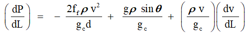
The energy balance for gas/liquid flow in either a horizontal or vertical conduit is provided as Equation 1 in its Pressure Gradient form. Figure 1 provides a visual reference for the dimensional criteria for the injected casing gas, or gas/oil flow from the producing Horizon “Pay zone”.
1 [3]
 1 [3]
1 [3]Flowing Pressure Friction Head Momentum
Gradient Gradient Gradient Gradient
NOTE: With due consideration, the units selected for the Gas Lift written material will be in FPS units. Conversion factors will be included for assisting the reader. Values will be provided in convenient units to yield appropriate results.
Where:
dP/dL = Pressure gradient lbf/ft2ft (psi/ft): (Pa/m)
ρ = Density of flowing phase: Single phase gas or two-phase gas/oil – water: lbm/ft3 (kgm/m3)
v = Velocity of flowing phase: Single phase gas or two-phase gas/oil – water: ft/sec (m/sec)
d = Diameter of production tubing for gas/oil-water flow; Equivalent annular diameter for Casing-tubing annular flow: IDcsg – OD tbg: ft (m)
Ɵ = Well production string angle; (for vertical; Ɵ = 90° (Sine Ɵ = 1))
gc = Gravitational mass - force constant: 32.2 lbm ft/sec2lbf (1 kgm m/sec2N)
g = Gravitational acceleration, 32.2 ft/sec2
ff = Fanning (Moody) friction factor from Reynolds Number, Re, taken from Moody Friction Factor Chart,
ρ = Density of the flowing Fluid: 1) Injected casing gas, 2) Production tubing Oil, Formation Gas (GOR)), and Injection Gas Oil Ratio IGOR, giving the total Gas Liquid Ratio or GLR (SCF/STB): lbm/ft3 (kg/m3)
The Reynolds Number, for use with the Moody Friction Factor Chart is defined as follows
2 [3]
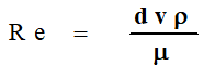 2 [3]
2 [3]Where: Terms are defined above.
The fluid viscosity, μ, is defined by the slope of the “Shear Stress” vs “Shear Rate” correlation. The units of viscosity are: 1 cp = .001 kg/m sec = 6.72 E-4 lbm/ftsec.
All terms related to the pressure gradient are in an energy base of: lbf/ft2ft, or the SI equivalent per unit mass (N/m2m). Proper conversions can be easily applied to convert the flowing gradient to typical units of: lbf/in2ft: Pa/m. Notice the first term is the friction gradient, referred to as the Darcy Equation. The “f” parameter is the basic Fanning friction factor that is applicable to the Darcy friction loss term. If selected from the Moody Reynolds Number correlation, the Fanning ff is the Moody value divided by 4 [3]. The “height” term is represented by the second gradient, which includes the Sine function to consider a non-vertical flow path while the last term is the momentum gradient.
Numerical computations have shown that the momentum component pressure loss does not play a large part in the gradient calculations both for single phase gas, or two phase gas/oil. Thus, the total pressure loss considered is designated by the Friction, and Head Gradients.
In terms of a flowing gradient: (dP/dL); psi/ft (kPa/m), the collected terms are dependent on the density, lbm/ft3 (kgm/m3) of the gas or two-phase gas-liquid, as well as the actual flowing gas, or oil/gas velocity, and “wetted” diameter of the flowing scenario. The total pressure gradient may be determined from these considerations.
II.B) The case of Casing/Tubing injected gas flow. An effective annular area must be
determined by:
AREAeff (in2) = Casing Inside Area (in2) – Production Tubing Outside Area (in2).
The fluid density term was taken from the standard equation for a gas, applying the following nominal range for the parameters as shown by Figures: A-2 – A-5.
Nominal “Average” Data Range for Vertical Gas Flow in a Gas Lift Well:
T - ºF 100 – 180 °F; Z = .85 - .95
P – psia 500 – 2500 psia: Gas Viscosity – cp .012 – .018
k (Cp/Cv) 1.23 – 1.24: MWg = 18.3 lb/lbmol
Table 1: Nominal parameters chosen for flow equations.
The following data were selected from Ref [4] reporting the commonly used Casing/Tubing dimensions employed in a Gas Lift well completion design:


1. Data: ENPRO (OCTG); Casing and Tubing, (OCTG Pipe) [4]
Table 2: Production Tubing, and Casing design parameters [4]
As discussed, the application of the flowing pressure gradient term requires an effective diameter and Area for tubing and casing. Flowing conditions also involve flow in the annulus between the casing and tubing. An “effective flow diameter” must be determined from the “effective area” exposed to the gas flow. Thus the effective annular areas, Aeff, and corresponding effective diameter, Deff, for the Casing–Tubing Configurations would be as follows:
Case 1: 9 5/8 in. Csg / 2 3/8 in. Tubing: Aeff1= .785{(8.681)2 – (2.375)2} = 54.76 in.2
Effective Diameter 1: Deff 1 = 8.35 in.
Case 2: 9 5/8 in. Csg / 2 7/8 in. Tubing: Aeff1= .785{(8.681)2 – (2.875)2} = 52.70 in.2
Effective Diameter 2: Deff 2 = 8.19 in.
Case 3: 7 in. Csg / 2 3/8 in. Tubing : Aeff1= .785{(6.094)2 – (2.375)2} = 24.72 in.2
Effective Diameter 3: Deff 3 = 5.91 in.
Case 4: 7 in. Csg / 2 7/8 in. Tubing : Aeff2 = .785{(6.094)2 – (2.875)2} = 22.66 in.2
Effective Diameter 4: Deff 4 = 5.37 in.
Table 3: Casing – Tubing Configurations showing Effective Diameter and Area [4]
The physical dimensions chosen for the well completion will impact the Casing Gas injection rate due to a reduced flow area. This area is specified as an “Effective Area”, “Aeff” in.2. This reduced area will impact maximum flow in the casing/tubing annulus.
Excessive gas flow velocities are not recommended, as friction gradient increases rapidly, and impact optimal oil flow. As shown, flow from the surface to the final GLV would generally be a configuration of the above selections, depending on gas rates, and depth. All these conclusions are essentially based on the “assumptions” stated for the Casing / Tubing dimensions.
Equation 3 [3] indicates the “head” or hydrostatic term for a gas column, expressed in pressure terms, is given by:
ΔPgas = ρg(g/gc)ΔH 3 [3]
When integrated over a differential height, the static gas pressure at the bottom of a vertical column Can be calculated as:
P2 = P1es 4 [3]
Where :
P2 = Pressure at bottom of column - lbf/ft2
P1 = Pressure at top of column – lbf/ft2
e = Naperian Log base : 2.718
s = Correlating function : ΔHγg/ATmzm
ΔH = Height differential – ft
γg = Gas gravity
Tm = mean absolute temperature – °R
Zm = mean value for z.
Fortunately, the generalized equation for computing the total flowing gas gradient in a conduit at “median” conditions for all fluid dependent terms, including the vertical head term are available. We have defined a simple and direct approach via:
5 [3]
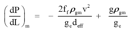 5 [3]
5 [3]To further simplify the actual calculations, an assumption has been made to determine the Moody friction factor by a simplified equation for f, assuming turbulent flow. This equation is based on small pipes [3]. It has been sparingly used in gas flow “f” factors; however in most Gas Lift cases, the injected casing gas is in the turbulent flow range, and resulting fMOODY , evaluated for small conduits (3” – 8”) is assumed to be applicable: For application of the flowing gradient equation, the Fanning friction factor ff is applied. The Fanning friction, ff, factor is the fMOODY divided by 4.
fMOODY = 4 x 0.0239(Re- 0.134) 6 [3]
The calculation procedure will be based on the follow the sequences:
II B.1) Calculation of flowing Gas gradients:
Curves are presented in Appendix A showing the flowing casing gas annular flow pressure gradient, (dP/dH)csg in psi/ft for the following sequence of data :
Series 1: 9 5/8” Casing with 2 3/8” production tubing
Series 2: 9 5/8” Casing with 2 7/8” production tubing
Series 3: 7 ” Liner with 2 3/8” production tubing
Series 4: 7 “ Liner with 2 7/8” production tubing
The gradient data will be simplified for the casing/tubing gas flow indicated by the following input flowing physical properties, and conditions:
- Surface Injection Pressure = 500, 1000, 1500, 2000, 2500 psi
- Flowing temperature range = 100 – 180 °F
- Mean “ z” factor = 0.88
- Molecular Wt. Gas = 18.3 lb/lbmol
- Mean Gas Viscosity = .014 cp (9.4 E-6 lbm/ftsec) ; ( 1.4 E-5 kgm/msec)
- Aeff, Deff = Effective Casing-Tubing Flow Areas (in2), and Diameter, Deff, (in.) for annular flow yielding an equivalent effective “flow area” are taken from Table 3.
- Selected Flow Range : 0.5 – 2.5 MMSCFD
As can be surmised, the gradient flowing parameters for pressure “gain” in the existing Casing/Tubing annulus must be known as this information yields the existing pressure at depth of the final (lowest) orifice Gas Lift Valve, shown in Figure 2.
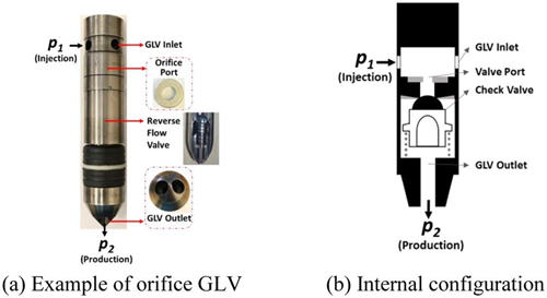
Figure 2: Bottom Hole Production Tubing Gas Lift Valve [6]
Notice from the presented data, that a reasonable pressure gradient range is duly established by Figures [A.1] through [A.4], Appendix A. As shown by the Figures, the flowing gradients range discreetly between 0.01 and 0.06 psi/ft. For a set casing/liner size, (either 9 5/8” or 7”), the production tubing diameter, i.e. from 2 3/8” to 2 7/8” will impact flowing gradients. The shown “Effective Area, and Diameter” are seen to decrease discretely, showing a slight increase in the flowing gradient. It is interesting, and important to note that beyond a casing injection rate of 0.5 MMSCF/D, the flowing gradient shows to be essentially constant. This occurrence is due to the impact of the flowing gas density term which is included in the friction loss portion of the gradient with a negative sign, and also is part of the corresponding increase of the static gradient which is positive. The curves should be very applicable when estimating the Casing gas injection pressure as illustrated by the following example:
Example 1: Gas Lift Well - Casing / Production Tubing Gas Injection:
a) Depth of pay zone in candidate well: 8000 ft.
b) Csg/Tbg upper completion: 9 5/8” x 2/3/8”: Depth: 7000 ft.
c) Liner/Tbg. Lower completion: 7” x 2 3/8”: Depth: 8000 ft.
d) Injection Gas Rate : 1.5 MMSC/D
e) Well Head Injection Pressure, and Temperature: 1500 psia, : 140 °F
f) Mean Z factor : 0.85
g) Mean gas viscosity: 0.015 cp.
h) Mol. Wt. Gas : 18.3 lb/lbmol
1) Solution :
a) Gradient in 9 5/8” x 2/3/8”annulus : 0.035 psi/ft (Figure A-1)
b) Flowing Pressure at 7000 ft. : 1500 + (0.035)(7000) = 1745 psia
c) Gradient in 7”x 2 3/8” annulus: 0.038 psi/ft (Figure A-3)
d) Production Tubing Valve Injection Pressure: = 1745 +(0.038)(1000) = 1783 psia
With these pressure vs depth data, and a knowledge of the well’s formation IPR, as well as the Solution Gas Oil Ratio (GOR – SCF/STB) of the formation fluid, the conditions are now set for a selection of the proper ORIFICE SIZE to be installed in the Production Tubing GLV.
II C) Consideration of Basic Orifice Flow as applied to an operational Gas Lift Valve (GLV)
To consider the fundamental conditions governing “orifice” flow, the basic energy balance is once again addressed. However, for the orifice flow case, the equation does not include the “friction loss” term, or the “head” term. The equation now considers the “pressure change” solely as a function of the momentum term:
7 [3]
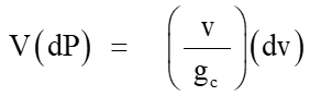 7 [3]
7 [3]For the specific case of an assumed adiabatic reversible (isentropic) expansion, pressure and specific volume V, (ft3/lbm), and pressure (lbf/ft2) are related by:
PVk = Constant 8 [3]
In Equation 8, the exponent, k, is the ratio of specific heats, Cp/Cv. With this assumption, the pressure loss across a restriction “choke”, could be fully recovered and downstream pressure would equal upstream pressure. In reality, some energy is lost to friction and the process is not reversible. Typically, this non-ideal behavior is resolved by assuming ideal behavior, then applying a correction factor to the result, which is the approach we will use here. The Thornhill – Craver relationship, Equation 11, applies this concept with the inclusion of the Cd factor. Alternatively, the exponent can be modified to better represent reality (such that “k” is not equal to Cp/Cv). In the latter case, the exponent is often determined experimentally, and is often referred to as the “polytropic” exponent. Either approach allows us to consider the case where the recovery of the upstream pressure is not reached due to some “polytropic” effect. The magnitude of the deviation is very dependent on the precise physical configuration of choke internals.
Notice in Figure 3, [5] depicting an orifice (choke) in a flowing condition, that the exchange of energy results in an increased “velocity”, and reduction of pressure for the fluid as it passes through the choke (orifice). The point of minimum pressure is termed the “Vena Contracta”. When the downstream area increases, the flow velocity decreases, and flowing pressure recovers; however due to the polytropic (i.e. non-ideal) conditions the recovering pressure does not reach the inlet value. This is the polytropic “energy loss”.
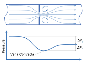
Figure 3: Flow through an orifice (choke) for ploytropic conditions [5]
Equation 9 now becomes:
[3]
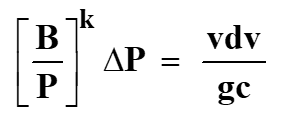 [3]
[3]This is the basis for most choke performance analyses, relationships, and working equations. This relationship yields the equations applied by Gilbert [6], Fortunati [7], and others. The fluid velocity, v, (ft/sec) can be related mathematically to the pressure differential, or pressure ratio across the choke.
The importance of all these solutions is the fact that a plot of downstream to upstream pressure ratios for choke flow: P2/P1 yields the application for fluid flow deemed the “transient, subcritical” flow regime. As shown by Figure 4 [8], for a given upstream pressure, P1, the flow increases across the orifice as downstream pressure, P2 is reduced, until further reduction of P2 will no longer increase flow. The reason for this behavior is that pressure disturbances are transmitted “upstream” at the speed of sound. Thus, when this velocity of the fluid at the vena contracts reaches the speed of sound, no additional flow is possible. This is referred to as CRITICAL flow. In this case, the “critical pressure ratio” is reported as 0.588, however this value is not a constant for typical natural gas flow through a choke. The critical pressure ratio varies from approximately 0.49 to 0.59.
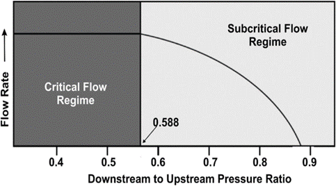
Figure 4: (P2/P1):
in an Orifice, or Choke [6]
For the purpose of this document, the Thornhill-Craver [2] Choke flow relationship has been applied. This relationship addresses the non-ideal (non-reversible) behavior in part by applying a correction factor, in this case, CD, the discharge coefficient which is derived experimentally.
In many Gas Lift instances, the calculated “choke capacity” has been well matched by this relationship. Equation 11 is the standard Thornhill-Carver giving a choke (orifice) capacity in SCF/d with all the parameters involved in the polytropic energy flow relationship. Appendix B presents the choke capacity results for various cases that coincide with the Flowing gradient curves with Appendix A. The selected data ranges are:
Upstream Pressures : 1000, 1500, 2000, 2500 psia
Choke Diameters : 0.125” (8/64ths”), 0.25” (16/64ths”), .375” (24/64ths”), .50” (32/64ths”)
Inlet Temperatures: 150, 175, 200, 225 °F
Gas Gravity : 0.63 (constant) – MW = 18.3 lb/lbmol
Z = .87 - .88 -.89 : k = 1.235 , 124 , 1.25 , 1.26
Equation 11, the Thornhill – Craver correlation will compute the specific choke capacity as a function of Pressure Ratios related to choke flow: P2/P1, downstream / upstream. The Figures in Appendix B show the flowing gas capacity as a function of the pressure ratio. All cases are seen to show the decrease in pressure ratio with increase in flow UNTIL the critical point is reached. This value is in the range of 0.55 - 0.48. Thus, once a bottom hole injection pressure has been determined, the choke must be selected to coincide in capacity (SCF/D) within its acceptable “sub critical” flow regime.
Equation 11 [2] is the Thornhill-Craver for Choke Flow through an orifice.
11 [2]
 11 [2]
Where:
Qg
=
gas-flow rate at standard conditions (14.7 psia and 60°F), Mscf/D,
Cd
=
discharge coefficient (determined experimentally), dimensionless,
A
=
area of orifice or choke open to gas flow, in.2,
P1
=
gas pressure upstream of an orifice or choke, psia,
P2
=
gas pressure downstream of an orifice or choke, psia,
g
=
acceleration because of gravity, 32.2 ft/sec2,
k
=
ratio of specific heats (Cp/Cv), dimensionless,
T1
=
upstream gas temperature, °R,
Fdu
=
pressure ratio, P2/P1, consistent absolute units
The correlations presented will allow the reader, and designer of a Gas-Lift well/system to choose a proper choke based on the flowing predictions for 8, 16, 24, and 32/64ths in chokes. The selected data will be displayed on the graphs. Rarely have choke performance curves been presented in this fashion, and their applicability is proven in that at the critical pressure ratio, at approaching sonic velocity, can be shown to exist. This critical pressure ratio has been shown to be expressed by:
12 [2]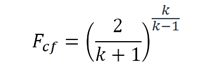 12 [2]
Where :
Fcf = Critical Orifice pressure ratio: P2(vena contracta) / P1 (inlet )
k = Specific heat ratio: Cp / Cv
All assumed parameters have been chosen to represent actual Gas Lift wells in the field. Further, the parameters are extended so the impact of critical flow can be seen.to.
If the previous example is revisited:
Example 2: Gas Lift Well - Casing / Production Tubing Choke Capacity:
a. Depth of pay zone in candidate well: 8000 ft.
b. Csg/Tbg upper completion: 9 5/8” x 2/3/8”: Depth: 7000 ft.
c. Liner/Tbg. lower completion: 7” x 2 3/8”: Depth: 8000 ft.
d. Injection Gas Rate : 1.5 MMSC/D
e. Casing Injection Pressure = 1500 psia
Solution:
Flowing pressure at Production Tubing/ 7” Liner depth is found to be: 1873 psia
Referring to Appendix B, two (2) Choke Dimensions are seen to provide the desired solution for the correct flowing bottom hole liner/tubing capacity in the orifice valves shown as follows:

As shown from the solution, both a 16/64 ths, or 24/64ths Choke will perform adequately. Perhaps the larger size, 24/64ths is the correct solution, as the remaining subcritical flow regime is greater: 0.96 - 0.5. This will allow for more casing gas to be injected, and provides leeway for corresponding increases, or reductions to the choke inlet pressure as flow conditions develop.
Summary:
In this Tip of The Month an analysis was performed in Section II A to review energy and mass balances as related to a candidate Gas Lift Well’s flowing gradients. Standard Energy balance equations provided the proper data to simulate both the annular flow in a casing/ tubing configuration, as well as for choke performance where energy change was related to momentum differential.
In Section II B, Casing/Liner, and Tubing sizes were selected to perform the necessary flowing gradients for the injected casing gas. Equipment Data recompiled from Industry standards provided the necessary injected Casing/Tubing/Liner dimensions to calculate Effective Areas, as well as Effective Diameters for flow of the injected casing gas to the Production Tubing Gas Lift Valve at a given depth.
Section II C reviewed the existing Industry standards for Gas Lift Choke flow. The Thornhill–Carver equation provided the choke performance data relating to the selected choke sizes. An example was presented to provide a flowing liner/tubing bottom hole pressure from the Gradient curves presented in Appendix A. The Choke performance curves in Appendix B were employed to “size” the proper choke diameter, and flowing conditions. The Appendix B curves apply to orifice sizing but are only an estimate for gas lift valves since the valve stem in the seat reduces flow area.
To learn more about similar cases and how to minimize operational problems, we suggest attending the G-4 Gas Conditioning and Processing Course presented worldwide. In addition, our session in ALS (Artificial Lift Systems), GLI, Gas Lift, and Completion and Workover courses.
By: Frank E. Ashford, Ph.D.
Wes H. Wright
The Authors would like to cite and appreciate the support received from Mr. John Martinez, PetroSkills Senior Advisor. Mr. Martinez is a known expert in Gas Lift applications. His excellent technical expertise, and proven field knowledge are reflected throughout this document. We also acknowledge and express our gratitude to Kindra Snow-McGregor for her valuable review and feedback.
References:
1. Simplified and Rapid Method For Determining Flow Characteristics of Gas Lift Valves (GLV); Mehdi Abbaszadeh Shahri: Texas Tech University, Aug. 2011
2. Cook, H. L. and Dotterweich, F.H. 1946 Report on Calibration of Positive Flow Beans manufactured by the Thornhill – Craver Company, Houston, Tx.
3. Gas Conditioning and Processing: The Basic Principles: (John M. Campbell): Vol 1 9th Edition. Editors R.A. Hubbard, K.S. McGregor
4. ENPRO (OCTG); Casing and Tubing, (OCTG Pipe) : (data and dimensions)
5. NEUTRIUM: Calculations of Flow through Nozzles and Orifices ; Feb. 11 , 2015
6. ELSEVIER: Flow Measurement and Instrumentation: Vol 76, Dec. 2020 – David A. Wood , et. Al.
Appendix A : Casing – Production Tubing Flowing Gradients

Figure A.1: Injected Gas Flowing Gradients in 9 5/8” Casing and 2 3/8” Production Tubing

Figure A.2: Injected Gas Flowing Gradients in 9 5/8” Casing and 2 7/8” Production Tubing

Figure A.3: Injected Gas Flowing Gradients in 7 ” Liner and 2 3/8” Production Tubing

Figure A.4: Injected Gas Flowing Gradients in 7 ” Liner and 2 7/8” Production Tubing

Figure B.1: Gas Lift Choke Performance: .125 in. ( 8/64”) Choke Diameter

Figure B.2: Gas Lift Choke Performance: .25 in. ( 16/64”) Choke Diameter

Figure B.3: Gas Lift Choke Performance: .375 in. ( 24/64”) Choke Diameter

Figure B.4: Gas Lift Choke Performance: .50 in. ( 32/64”) Choke Diameter